Blueprints for BI Data Modeling: Star, RLS, and SCDs in Action

Introduction

Designing a BI semantic layer is not just about theory. You’ve probably heard of Star, Snowflake, or Data Vault (if not, read about them here), and maybe even the different types of fact tables in Kimball or OLAP modeling articles. But when it comes to production-grade models in Power BI, SSAS, AAS, or Microsoft Fabric, what you really need are blueprints 📘.

This article focuses on Kimball modeling and the Power BI ecosystem, but many of the modeling paradigms described here can be ported beyond Power BI into other BI and OLAP platforms.

In this article, we’ll explore a series of blueprints that leverage advanced patterns such as Hybrid Models, Benchmarking, and Row-Level Security (RLS). Each blueprint is designed with a clear purpose, recommended use cases, and highlights of common pitfalls to avoid.

Because at the end of the day, BI modeling is not academic, it’s pragmatic 🧐! The best models are not the most elegant on paper, they are the ones that survive in production.

General best practices

Before we dive into the blueprints — what to do and what not to do — let’s start by laying down some foundations. These are the general practices every model should respect, no matter the scenario:

• Model scope, one data model equals one business story.
• Grain first, define and document the fact grain. One row equals one event.
• Surrogate keys in dimensions, for example customer_sk, keep business keys like customer_id or customer_local_id only for lineage..
• Date Table, always create a proper calendar table, disable Auto Date/Time, and use it as a common slicer across multiple tables.
• No many to many, resolve N to N with a bridge or a factless fact.
• Relationships, prefer single direction filters, use bidirectional only in narrow and controlled cases, otherwise you risk circular filters.
• Inactive relationships, keep them rare, activate with USERELATIONSHIP only when needed.
• RLS, apply on dimensions, never on facts, let RLS propagate through active relationships.
• Compression, think per table and per column, avoid high cardinality columns and duplicated tables, duplicates do not compress again.
• Measures over calculated columns, push shaping to Power Query, keep DAX for measures.
• Data types, choose the smallest type that fits, use whole numbers for keys, avoid GUIDs in facts, cardinality is high and compression is poor.
• Incremental refresh and partitions, partition large facts by date or by a dimension such as country, define RangeStart and RangeEnd.
• Naming and organization, consistent DimX and FactY, keep a dedicated measures table, use display folders.

Some Perquisites

Before we get into the blueprints, there are a few prerequisites worth aligning on. These are the building blocks that come back again and again in real-world models.

Fact tables types

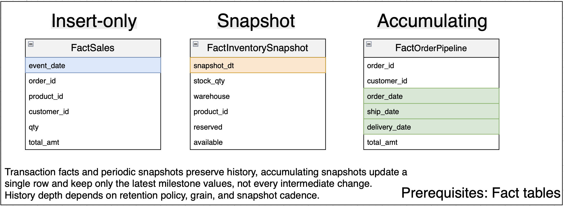
Kimball defines three fact table types you will see most often:

• Insert only, Transaction Fact, grain equals one row per business event, sale, payment, click. Rows are inserted once and never updated. Ideal for auditing and drilling to atomic detail.
• Periodic Snapshot Fact, grain equals one row per entity per snapshot date, daily balance, monthly stock. Insert on a fixed schedule to record state at a point in time. Best for trends and time based KPIs.
• Accumulating Snapshot Fact, grain equals one row per process instance, order, claim, ticket. Add or update columns as milestones complete, missing milestones are NULL until reached. Good for pipeline and SLA tracking.

👉 For a deeper dive, see, Masterclass Data Modeling – How Data Changes Drive Schema Design.

Dim tables and SCDs

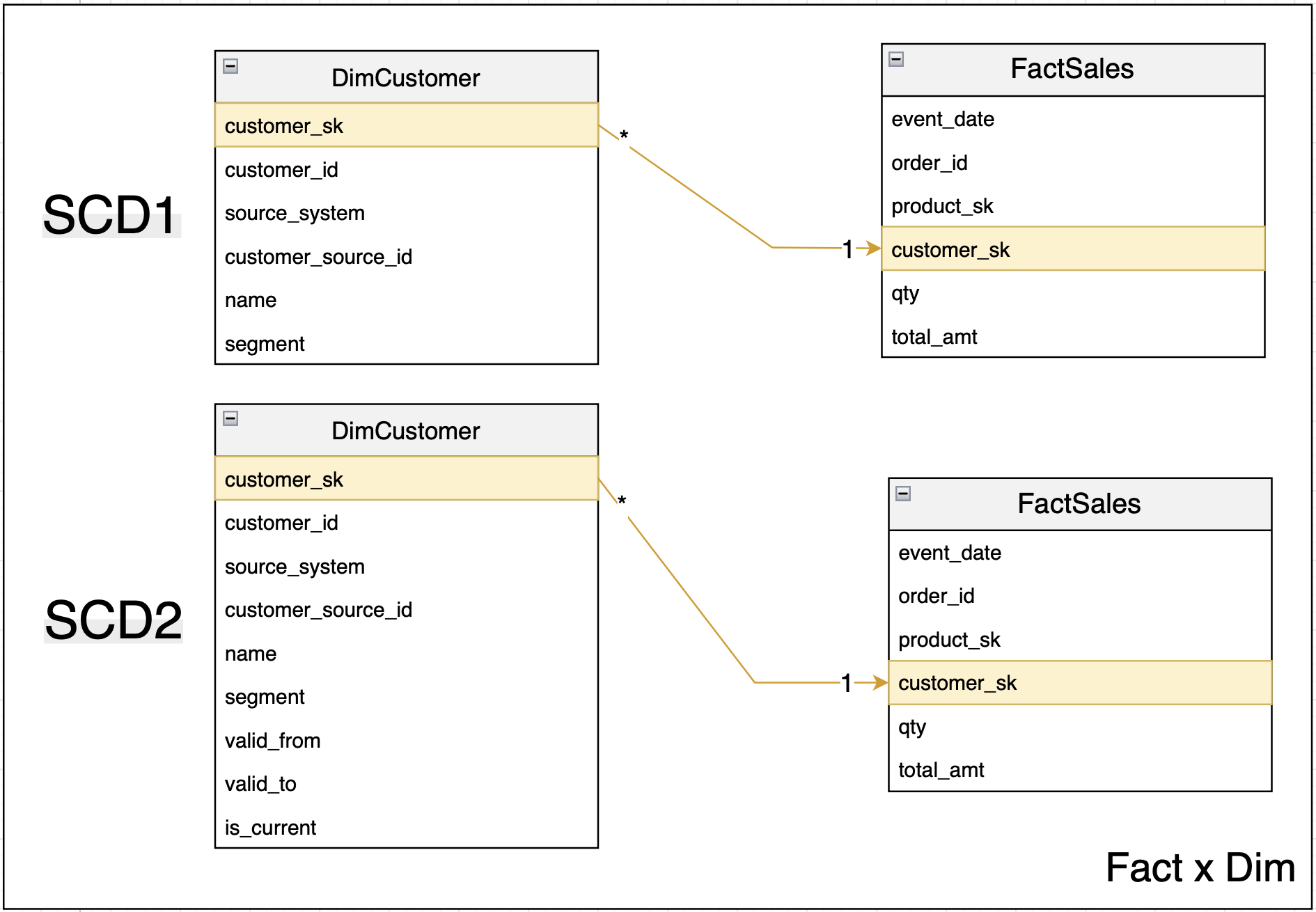
If you want a general overview of SCDs — what they are and how they work — I suggest checking the article I referenced earlier. Here, I’ll focus only on the dimension types you actually see the most in BI models: SCD1 (keep latest value) and SCD2 (keep historical).

Why? Because SCD0 is just a static table that never changes (so the join is straightforward). SCD4 can be used, but only if you pre-process and join the current and history tables before consumption. SCD3 is sometimes used to keep and display the previous value, but its use is very limited for BI since it doesn’t support drill-down or flexible joins. And SCD6 is more of a hybrid mix-and-match, very rarely implemented in real-world projects.

Keys, rules that always apply

• Every dimension gets a surrogate key, SK, for SCD1 and SCD2.
• SKs are warehouse generated, meaningless, immutable, unique, never reused.
• Facts store only SKs, never business keys.
• Keep business keys, BK, in the dimension for lineage and uniqueness, for example customer_id or the pair (source_system, customer_local_id).
• For SCD2 changes, insert a new row with a new SK, keep the same BK, never update or reuse SKs.

How keys flow across layers

• Bronze: Store data as received, keep only BKs, do not create SKs.
• Silver: Deduplicate on BKs, detect SCD2, assign SKs, keep both SK and BK, SK is for joins, BK is for lineage and change detection.
• Gold: Facts store only SKs, dimensions expose SK and BK, joins are SK to SK, SCD2 version selection is handled in Silver, no point in time logic in DAX.

Blueprint Catalog

Globally, you’ve probably read about Star schemas, Snowflakes, or Galaxies in the books. That’s fine for theory. But the reality in production is much messier. Instead of giving you 50 lectures, we’ll focus on a set of blueprints you can actually use — solid, proven, and directly applicable. That’s where we’re heading 🚀 !

#1: Fact KPI tracking

The business goal of this model is to track sales KPIs and operational performance across detail and aggregate levels. This model uses a pragmatic star with a light snowflake (or galaxy if you use aggregate), FactSales is append only for transactions, FactSales_Aggregated is a pre-aggregated import table, Product is SCD2 and Date is conformed.

Implementation notes:

• Keep the tuple small, in FactKPIsProduct_Aggregated include only slice dimensions you need, for example date_key, supplier_sk, store_sk, don’t use order_line_id (the smallest grain) because it will kill the aggregation.
• Store additive totals, not averages, keep sum_quantity, sum_net_amount, sum_discount_amount, optionally sum_gross_amount. Storing non-additive totals is wrong ! Averages of averages (without weight) doesn’t have any sense.
• Aggregations setup, declare the grouping tuple on FactSales_Aggregated, set those dimensions to Dual, make sure the detail table uses the same keys and that they are active relationship between the aggregation table and the dimension tables.

#2: Dimension KPI tracking

The business goal of this model is to track data quality and operational KPIs for the Product dimension. This model follows a pragmatic star with a light snowflake (or galaxy if you use aggregate), where Product is SCD2, Date is conformed, and KPIs are captured in a periodic snapshot FactKPIsProduct_Snapshot with fast reporting served by an Import aggregated table FactKPIsProduct_Aggregated.

Implementation notes:

• Keep the tuple small, in FactKPIsProduct_Aggregated include only slice dimensions you need, for example date_key, supplier_sk, subtype_sk, don’t use product_sk (the smallest grain) because it will kill the aggregation.
• Metrics are additive, in the snapshot store 0/1 flags and optional numerators and denominators, in the aggregated fact store sums only, compute rates as weighted averages in measures, never store pre averaged values.
• Aggregations setup, declare the grouping tuple on FactSales_Aggregated, set those dimensions to Dual, make sure the detail table uses the same keys and that they are active relationship between the aggregation table and the dimension tables.

#3: 2 Facts Tables

The business goal of this model is to track sales performance and inventory availability across stores and products. The model follows a pragmatic star with a light snowflake, where Product and Store are managed as SCD2 dimensions to preserve historical accuracy, Date is a conformed dimension used across all facts, and business processes are separated into two complementary facts: FactSales as an append-only transaction fact for revenue and margin analysis, and FactInventory as a periodic snapshot fact for stock levels.

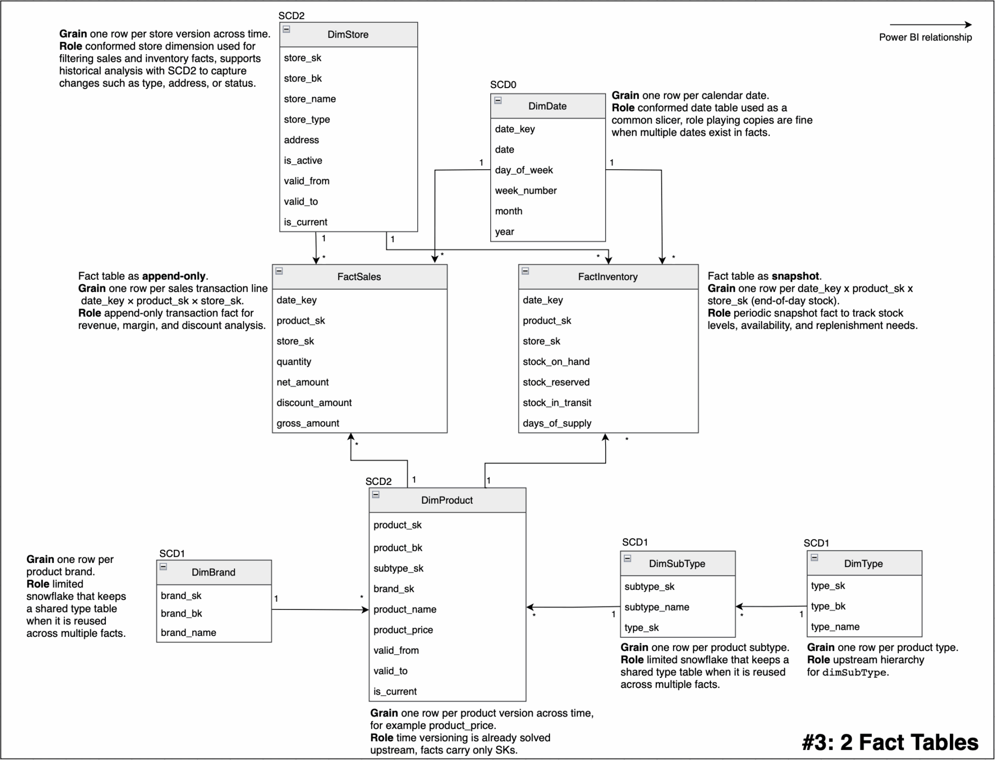
Implementation notes:

• Use additive measures only in facts (quantities, net_amount, stock_on_hand). Derived ratios such as sell-through or stock-to-sales should be calculated in measures, never pre-stored.
• For performance, you can set up aggregated tables (for example, daily product-store sales) and configure them as Dual in BI tools, ensuring consistent surrogate key usage and active relationships with shared dimensions.

#4: Benchmarking (with RLS)

The business goal of this model is to let a region restricted user, for example France, analyze their secured sales while benchmarking against worldwide totals. The model duplicates the sales fact into a protected path, FactSales, and an unsecured reference path, FactSales_no_rls.

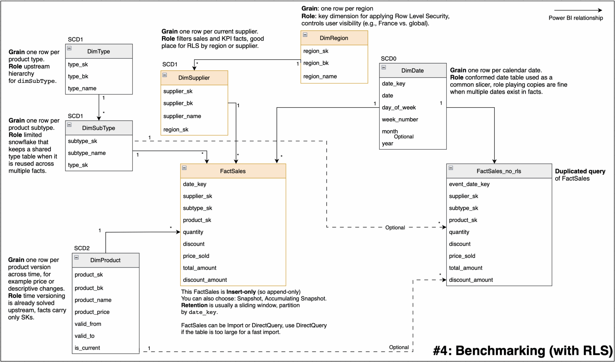
Implementation notes:

• Size warning, duplicating the fact costs memory, VertiPaq compression happens inside each table, so FactSales_no_rlsroughly doubles storage.
• Where to put RLS, define RLS only on DimRegion or an authorization table that filters DimRegion, do not define RLS on Supplier, on any bridge, or on FactSales_no_rls.
• Relationships and slicers, keep FactSales active to Date, Product, Supplier, Region, for FactSales_no_rls, either keep no relationships, which gives a static global comparator, or relate only to Date and Product, since they are not RLS filtered.
• Do not relate Supplier, the filter will propagate and you will lose the global non RLS behavior! If you also need Supplier on the world figure use USERRELATIONSHIP or TREATAS on duplicated columns (you have to create them!), as a last resort you can connect Supplier to FactSales_no_rls with a *-1 direction where the fact is on the 1 side, which by default does not carry RLS (I tried it in real life, not very elegant, but works!).

#5: Anti-patterns

To introduce the topic, we will first show a large model that includes everything not to do, each anti pattern will be numbered, and the notes below will explain every number.

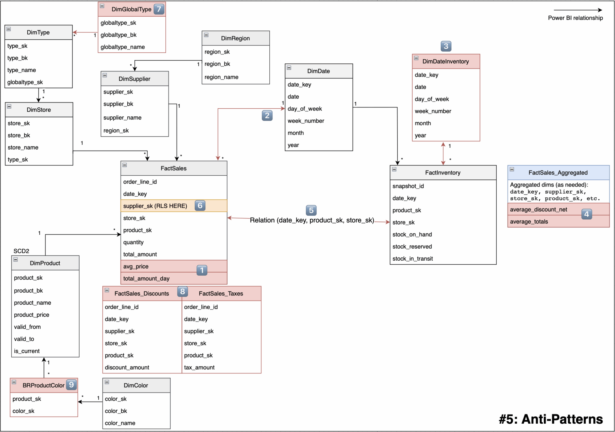
Pitfalls in this model:

• 1️⃣ Do not mix grains in a fact table, keep only transaction rows, move pre-aggregated rows to a separate _Aggregated table or remove them.
• 2️⃣ Do not use bidirectional relationships (until needed), they cause unpredictable filter propagation and can break RLS.
• 3️⃣ Non conformed Date, two separate date tables, slicers do not filter both facts consistently, time intelligence is inconsistent.
• 4️⃣ Non additive metric stored in a fact, average_totals is a rate, it must be computed as a weighted measure.
• 5️⃣ Many to many between FactSales and FactInventory, creating a direct M:M link between two facts introduces ambiguous filter paths, double counting, cardinality blow up, unpredictable totals, and possible RLS leakage.
• 6️⃣ RLS defined on a fact table like in supplier_sk, expensive, fragile, easy to bypass through other paths.
• 7️⃣ Over snowflaked hierarchy, DimGlobalType → DimType → DimStore → FactSales , long chain to the facts. Thus, too many joins, slow performance, complex filters. Snowflake dim tables had to be flatten out.
• 8️⃣ Multiple fact tables for one process at the same grain cause redundant joins, inconsistent filters, duplicated RLS and measures, and poor per table compression, slowing queries and skewing totals. Consolidate into a single FactSales at one grain.
• 9️⃣ Bridges that forces duplication, this is more a warning than a real anti-pattern because using a bridge is the correct way, but keep in mind that a bridge can create false calculations. Suppose Shirt A is red and blue, Shirt B is blue. If you select all the Colors, now you get 3 articles (instead of 2), so the sales will be 2x [Shirt A] + 1x [Shirt B], which is wrong. To fix this, you use DISTINCTCOUNT or REMOVEFILTERS carefully in your DAX.

Conclusion

🎉 With that, we are done with BI patterns and anti-patterns, especially in Power BI.

Just a reminder, nobody cares if your thing is super technical or shiny ✨. Complexity is not a badge of honor, it is a maintenance cost. If it is complex, you are probably the only person who understands it today, and in three months no one will, including future you 🙃. Aim for clear names, simple flows, and boring solutions that survive handovers and audits.

👉 Want to go deeper into the story and how Power BI actually works? Check out the full walkthrough article.