

In the global overview, we explored how the Data Lakehouse combines the robustness of a Data Warehouse with the flexibility of a Data Lake. Now let’s go deeper to understand how it works, what patterns it supports, which tools are used, and what the limitations of this architecture.
Quick Recap ↻
A Data Lakehouse builds on the foundation of a Data Lake 🛶 by adding core warehouse capabilities: transactional updates, schema enforcement, metadata management, performance optimizations, and governance.
Rather than maintaining two separate systems, a data warehouse and a data lake in a Hybrid Data Warehousing, a data lakehouse a unified platform that supports both use cases with a single storage layer.
Why was this architecture created?
Data Lakes offered flexibility and scale, but without structure or governance, many became swamps 🐸. Data Warehouses provided consistency and reliability, but lacked support for unstructured data or native real-time streams.
Hybrid Data Warehousing bridges the gap by maintaining both systems, but it introduces complexity: two storage layers, duplicated data, fragmented governance, and costly orchestration.
Thus, welcome the Lakehouse 👋 ! Instead of making users choose between flexibility or structure, Data Lakehouse utilizes open formats (so no vendor lock-in, you control your data 🛂!) and added layers of ACID transactions, schema enforcement, time travel, and governance directly on top of the Data Lake.
Let’s do some historical background: Databricks started back in 2013, originally as a commercial layer on top of Apache Spark (👪 one of Spark’s creators is also a co-founder of Databricks). For years, like most people running Spark on the cloud, they stored data in open format (Parquet) on object storage like S3, GCS or ADLS. It worked, but it lacked reliability: no transactions, no versioning, and schema issues were common.
Soon after, Databricks introduced Delta Lake and later open-sourced it, creating a little bomb in the industry 💣. It added key features like ACID transactions, schema enforcement, versioning, and time travel, fundamentally transforming how data lakes were used. Following that, Iceberg (by Netflix) and Hudi (by Uber) emerged, each addressing similar challenges in their own way, with different design choices around table management, performance, and integration.
Cloud platforms quickly began integrating these concepts. Traditional cloud data warehouses are evolving toward lakehouse features. For instance, Snowflake has integrated Iceberg, Google introduced BigLake, and Microsoft launched OneLake via Fabric. The lakehouse is no longer something experimental with uncertain effectiveness; instead, it has evolved into a first-class architecture for unified analytics, machine learning, and large-scale streaming.
Core Architectural Principles

Key Features of a Lakehouse

Data Lakehouse = Data Lake (object-based storage) + Data Warehouse (performance and management capabilities).
In a Lakehouse architecture, all data is stored in file formats on top of object-based storage, following the same approach as a data lake. However, it builds on this foundation by adding the key features and capabilities of a data warehouse.
This combination enables:
- ACID transactions & time travel for consistent reads/writes and access to historical data.
- Schema evolution to handle changes in data structure without rewriting datasets.
- Efficient querying through predicate pushdown, partitioning, V-ordering, and Z-ordering (we will write a technical article on this !).
- Streaming + batch support to unify real-time and historical processing.
- Compaction & vacuuming to manage small files and clean up obsolete data.
- Catalog & governance integration for centralized schema, access control, and lineage.
Storage and Table Formats
As we just said, a Lakehouse is built on top of object storage systems like S3, ADLS, or GCS (and to some extent, HDFS). Object storage allows data to be distributed across many machines, which is essential when dealing with massive datasets that simply can’t fit on a single server. It stores data as independent objects, each containing the content, metadata, and a unique identifier, making it both scalable and cost-effective for large-scale workloads.
INSERT, DELETE, or MERGE, critical for tasks such as fine-grained deletes, required by privacy laws like GDPR or CCPA. Without this, removing a single record could mean rewriting full files, which is inefficient and risky at scale.Cloud vs On-Prem
The data lakehouse is built for a cloud-native model. Why? Because cloud storage is cheap and scalable, while compute can scale up or down as needed. This flexibility reduces costs and adapts to changing workloads. Cloud platforms also provide built-in features like governance, metadata management, auto-scaling, and unified catalogs.
In contrast, building a Lakehouse on HDFS is possible but far from ideal: the setup is rigid, lacks modern integrations, and ends up closer to a hybrid between a Data Lake and a warehouse than a true Lakehouse.
Serving and Query Layer
Unlike traditional data warehouses, a data lakehouse separates storage from compute (like a data lake). This means you can scale them independently: use one set of machines to store the data, another to query it, and others to process it as needed.
Lakehouse processing relies on distributed compute engines such as Spark or Flink, which support both batch and streaming workloads at scale.
Why compute on multiple machines? Because if you want to apply a filter on a DataFrame, loading the data in RAM is 10-100 times faster than reading it from disk. And since we still haven’t seen a computer with 2TB of RAM, we distribute the processing and use MapReduce-style approaches, just like in a Data Lake.
Deep dive into layers
The Lakehouse layering model is not a brand-new invention, it is the classic data-warehouse pattern of staging → core → presentation reborn on object storage. Databricks simply popularised the idea under more marketable names bronze → silver → gold, and cloud providers quickly adopted the same tripartite flow in their own blueprints.
We will explore each of the three Lakehouse layers in detail, demonstrating how they transform raw data into valuable insights:
🟤 Bronze Layer
The Bronze Layer is the entry point of the lakehouse. It lands raw data exactly as received, applying only minimal technical hygiene. Data sources include OLTP systems (through CDC or extracts), IoT devices, event streaming platforms, REST APIs, or file like CSV, JSON, XML, or Parquet. Ingestion is orchestrated using tools such as Spark, Databricks Auto Loader, Delta Live Tables, Airflow, or dbt.
While the Lakehouse supports semi-structured and unstructured data, the Bronze Layer still mirrors many of the staging best practices from traditional ETL architectures:
- Immutable by design: Like in traditional staging layers, bronze data is append-only, versioned, and timestamped. This ensures auditability and safe reprocessing.
- Raw landing with minimal interference: Data is stored with its original structure. Only lightweight technical adjustments are allowed, such as type casting, dropping corrupt rows, format conversion (e.g., JSON to Parquet), or metadata tagging (e.g., ingestion time, source ID).
- Data contracts matter: Ingestion is often defined by data contracts, specifying schema, format, delivery time, and validation rules. These ensure consistency and can be enforced at runtime.
- Partitioned sources can be preserved or unified: Systems exposing partitioned tables (e.g.,
orders_2023,orders_2024, orinstore_orders,webshop_orders) can either be kept separate or consolidated into one logical table with metadata columns (e.g., year, channel) to retain traceability. - Unstructured data stays in Bronze: Files like images, PDFs, and videos are stored here permanently, referenced later via metadata tables but not transformed or propagated to upper layers.
Before data reaches Bronze, it is first staged in the Landing Zone, which acts as a raw file drop. This area is not part of the metastore and stores files exactly as received from the source systems. Examples of such paths include:
/landing/crm/customers/2024/03/02/customers.csv
/landing/crm/customers/2024/03/03/customers.csv
The Landing Zone enables full traceability, supports reprocessing, and serves as the system of record in case of ingestion failures or audits. After landing, all these daily files (e.g., .csv) are read and consolidated into a single managed table in the Bronze layer. Although physically stored in optimized formats like Parquet, this table is registered in the metastore (e.g., as a Delta table) and allows structured access, metadata tracking, and downstream processing..
⚪ Silver Layer
The Silver Layer transforms raw ingested data into technically validated, structured, and queryable datasets. It focuses on enforcing schema, improving data quality, and consolidating data from multiple sources. It turns raw input into cleansed, structured, and query-ready datasets. The Silver Layer is typically modeled in 3NF or as a Data Vault.
It is usually physically stored and organized into two sublayers, which can also be segmented by country, business unit, or other dimensions:
Prepared Layer
- Cleaned for technical consistency: column renaming, type casting, null handling, deduplication, basic constraints. No business rules are applied.
- Still source-aligned: for example,
customer_france,customer_germany,sales_physical_store, andsales_onlineare maintained separately. Limited regrouping may occur within the same source. - Optimized for lineage tracking, schema enforcement, and downstream reuse. Metadata like
source_systemandingestion_timeis added for traceability. - Supports incremental processing, schema evolution, and upserts using the previously discussed formats like Delta, Hudi, or Iceberg.
- Records that fail quality checks are redirected to a Quarantine Layer, which isolates invalid data without blocking the pipeline.
Unified Layer
The Unified Layer integrates and standardizes data across multiple source systems to create consolidated, business-ready entities. It introduces semantic consistency and historical tracking, forming the foundation of enterprise-wide analytics.
- Merges data from different systems into unified tables (e.g.,
customer,product,sales). It leverage merge operations (e.g.MERGE INTO) are used to update mutable records efficiently. - Introduces surrogate keys to replace conflicting or system-specific identifiers. It applies business logic, mappings, and reference joins.
- Reconciles semantic differences (e.g., aligning definitions of “revenue” or “status”).
- Normalizes codes and values across sources (e.g., “FR”, “France”, “FR01” →
country_code = 'FR'). - Leverages Master Data Management (MDM) when available, for golden records and identity resolution.
- Implements SCD2 (or other historization) techniques for mutable data (e.g., customers, products). It maintains
valid_from/valid_totimestamps for point-in-time analysis and traceability
🟡 Gold Layer
The Gold Layer materializes subject-specific data marts using denormalized tables, such as dimensional schemas (Star, Snowflake, Galaxy) or wide tables. This layer is optimized for business intelligence (BI) and downstream consumption.
Sometimes referred to as data marts, the Gold Layer may either include them directly or serve as a source for downstream marts. Its components can be implemented as either physical (materialized) tables or virtual (logical) views.
This layer can include:
- Domain-specific sublayers, tailored to business units such as Sales, Finance, or HR, providing curated facts and dimensions for targeted use within each unit.
- Product-specific sublayers, built around data products or specific analytics use cases, often accessed via APIs, dashboards, or self-service tools.
Business logic, KPIs, and aggregations are embedded to allow direct consumption (e.g., monthly revenue or churn rates). ML feature sets and training datasets are also built here, leveraging the layer’s curated structure. Exposure is typically through SQL endpoints, Delta Sharing, or semantic layers in BI tools like Power BI, Tableau, or Looker.
Nothing beats a real-life example 🧙
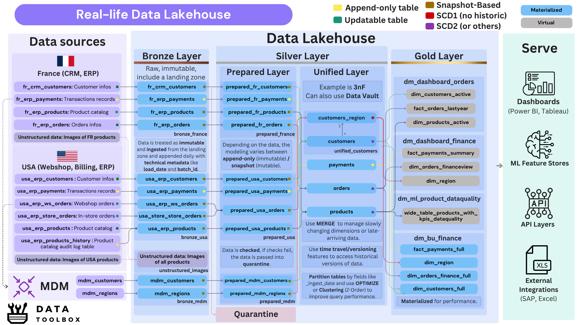
This is a dense and detailed diagram that provides an overview of a lakehouse architecture. It illustrates the full data lifecycle, from raw ingestion to data serving, while highlighting the various layers and transformations involved.
To fully grasp this canvas, you need a good understanding of data mutability (append-only vs. updatable), data modeling techniques (like 3NF or SCD), and a solid background in analytical versus transactional design.
Multi-Tenant vs Single-Tenant Lakehousing
As organizations scale their data infrastructure, choosing between multi-tenant and single-tenant lakehouse architectures becomes an important architectural decision. Each model comes with trade-offs in governance, scalability, and team autonomy.
- Multi-tenant lakehousing shares storage, compute, and catalog infrastructure across teams, using logical separation (namespaces, schemas, access controls) to manage isolation and governance. It improves efficiency but requires strict policy enforcement.
- Single-tenant lakehousing gives each team or domain its own independent lakehouse instance, with separate storage, catalogs, and compute. This ensures strong isolation and autonomy, allowing organizations to operate multiple lakehouses in parallel.
Today’s Technologies

As more traditional data warehouses adopt the marketing term “lakehouse” and implement some of its features, it’s important to clearly separate what’s real from what’s not, and understand what each platform is and what it really does.
- Lakehouse Platforms (Managed or Integrated Solutions)
- Databricks (✅ Lakehouse): Built on Delta Lake (open format), fully decouples storage (S3, ADLS, GCS) and compute (Spark, SQL, external engines). Supports batch, streaming, ML, BI workloads.
- Microsoft Fabric (✅ Lakehouse) : Uses OneLake and Delta Lake for unified lake-first storage, supports both SQL and Spark for analytics, and integrates tightly with Power BI for a seamless end-to-end experience.
- BigLake (✅ Lakehouse): Unifies BigQuery and Cloud Storage, supports open table formats like Iceberg and Delta, and offers serverless querying with integrated governance via Dataplex.
- Snowflake (🟡 Evolving) : Now supports Iceberg tables and Unistore. Still a mostly closed ecosystem with limited external engine access, but moving toward openness.
- BigQuery (❌ Warehouse with some lakehouse capacities): Supports structured and semi-structured data. Storage and compute are separate but tightly coupled to Google Cloud. Limited external engine support, with some lake access via BigLake.
- Redshift (❌ Warehouse with some lakehouse capacities) : Uses proprietary formats with tightly coupled compute/storage. Redshift Spectrum allows limited lake access but does not support open table formats like Iceberg or Delta.
- Synapse Analytics (❌ Warehouse) : Integrates SQL and Spark engines, with some lake connectivity (via ADLS), but lacks native support for open table formats.
- Table formats (view full comparison and details)
- Delta Lake: Uses a simple JSON transaction log and stores data in Parquet.
- Iceberg: Stores both metadata and data in Avro, and is optimized for real-time ingestion and incremental processing
- Hudi: Uses a manifest-based metadata model in Avro/JSON.
- Query engines
- Spark (Swiss Army knife 🛠️): supports batch, ML, and streaming workloads.
- Flink (Streaming-first ⚡): ideal for low-latency, real-time processing.
- Trino / Presto / Dremio (SQL engines 🔍): fast, interactive SQL queries over Iceberg, Delta, and Hudi.
- Hive / Impala (Legacy batch 🏚️): in-disk, still used in some Hadoop-based environments.
These ecosystems empower organizations to decouple storage and compute, enabling scalable, cost-efficient analytics.
To conclude, is this architecture still relevant?
Data Lakehouse architecture is a major milestone in the evolution of data platforms. While the learning curve can be steep, it pays off by enabling powerful, unified analytics and AI workloads.
That said, there are things to consider :
- Moving from classic SQL environments with stored procedures to a file-based, Spark engine can be challenging and may require rethinking your data processing approach.
- For highly structured, low-latency, high-concurrency workloads, traditional MPP data warehouses can still offer superior performance.
- Poor management of Delta tables (e.g. without regular vacuuming or compaction) can lead to performance and cost issues.
👉 Next up: Dive into Data Fabric or Data Mesh in our next architectural deep dives.