

Disclaimer
This article is part of a series, we highly recommend reading the following articles:
- The Foundation of a Scalable Data Architecture: Data Modeling 101
- Data Modeling: Dive into data normalization levels
These will provide the necessary context to fully grasp the concepts we discuss here.
Introduction
“Cause you’re a sky, full of stars, I’m gonna give my heart.” 🎶 While this may not be a standard way to begin a technical article, today we’ll be exploring the galaxies and the stars of data modeling 😁. Today we will analyze how different modeling techniques impact analytical workloads !
From Normalization to Analytics: A Shift in Paradigm
In our previous article, we discussed normalization levels, ranging from 1nF to 5nF, and highlighted why Boyce-Codd Normal Form (BCnF) is crucial for transactional workloads (specifically for relational databases). BCnF ensures data integrity and reduces redundancy, making it an essential design principle for OLTP systems.
What Changes in Analytical Workloads?
Analytical systems, unlike transactional ones, follow the Insert-Once, Read-Many paradigm, meaning they prioritize read performance over write efficiency. The key challenge in analytics is optimizing query performance, often at the price of increased storage usage and redundancy.
In OLAP environments, we often use columnar-oriented tables for storage and transmission (because they’re more efficient like Parquet, see this article !), and data models are designed to enhance aggregation, reporting, and query performance. This is where denormalized models shine, as they reduce the need for complex joins, making data retrieval much faster.
Common OLAP Modeling Techniques
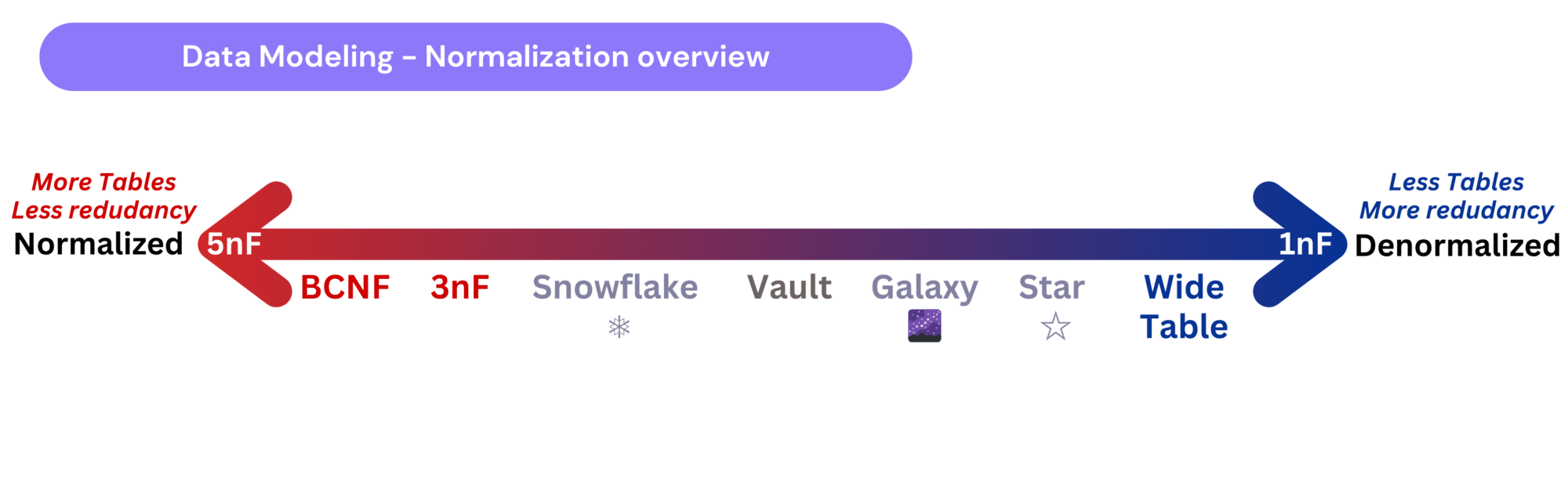
Let’s explore three key modeling approaches used in analytical workloads, ranked from the most denormalized to the least normalized.
Wide Table Schema
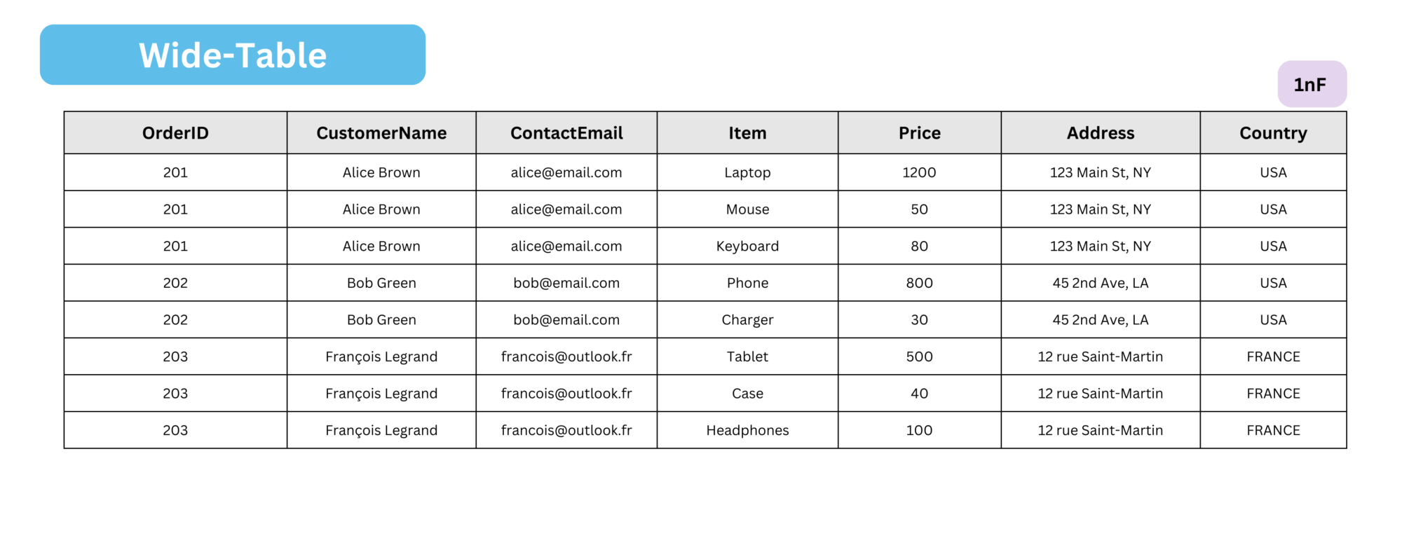
A wide table schema is the simplest form of denormalization. It stores all relevant data in a single table, significantly reducing the need for joins.
- Data is flattened into one large table.
- Simplifies queries since everything is stored together.
- Increases storage consumption due to redundancy.
In real-world scenarios, wide-table models aren’t very common. They usually appear in highly specialized cases that demand ultra-low latency or machine learning applications. This happens when the computational overhead of joining multiple tables becomes too costly.
Dimensional Modeling
Dimensional modeling structures data into fact tables and dimension tables, making it the standard approach for business intelligence (BI) and data warehousing. This methodology was pioneered by Ralph Kimball, a renowned data warehousing expert, whose approach emphasizes optimizing query performance and usability in BI systems. I personally recommend his book if you want to understand deeper: The Data Warehouse Toolkit: The Definitive Guide to Dimensional Modeling.
Core concepts of Kimball Modeling
General definitions:

Dimension Tables: Provide descriptive context to facts, such as time, product details, customer demographics, or locations. They enable filtering, grouping, and drilling into the data for analysis.

👉 Don't forget: In dimension tables, using a surrogate key (such as a UUID) is crucial for maintaining consistency and preventing key conflicts. Natural keys, which come directly from source systems, may not be unique across different data sources.

Fact Tables: Contain measurable business data, such as sales transactions, revenue, or quantities. They are central to analytical queries and include foreign keys linking to dimension tables.

✅ You need to explicitly choose the granularity of the fact table—that is, define exactly what each row represents (e.g., one sale per product per store per day). This decision sets the level of detail available for analysis, impacts how much storage you will need (therefore your AAS/SSAS cube capacity, or PBI cloud capacity), and must be made early, as it affects the design of related tables.

In-detail definitions:

Bridge Tables: resolve many-to-many (M:N) relationships.

Factless Fact Tables: records events or relationships but does not contain numeric measures (like event tracking).

Aggregated Fact Tables: Pre-summarized fact tables designed to improve query performance by storing data at higher levels of dimensional granularity. Can be used to reduce size of fact table in a gold layer or semantic layer of a dashboard. This higher-level granularity table is useful for storing summarized insights—such as trendlines or performance over time—when detailed transactional data isn't required.

Additive, Semi-Additive, and Non-Additive Facts:
• Additive Fact: A measure in a fact table that can be summed across all dimensions (e.g., Sales Amount, Units Sold) ➤ You can total it by day, product, region, etc.
• Semi-Additive Fact: A measure in a fact table that can be summed across some dimensions, but not all (e.g., Account Balance, Inventory Level) ➤ You can sum by product or region, but not reliably over time.
• Non-Additive Fact: A measure in a fact table that cannot be summed across any dimension (e.g., Ratios, Percentages, Rates) ➤ Averaging or other calculations are needed.

Data exploration techniques:
• Slicing: Selecting a specific subset of data by filtering on one dimension (e.g., sales in 2024).
• Dicing: Analyzing data from multiple dimensions by creating a smaller cube (e.g., sales by region and product).
• Drill-down: Navigating from summary data to more detailed levels (e.g., from yearly to monthly sales).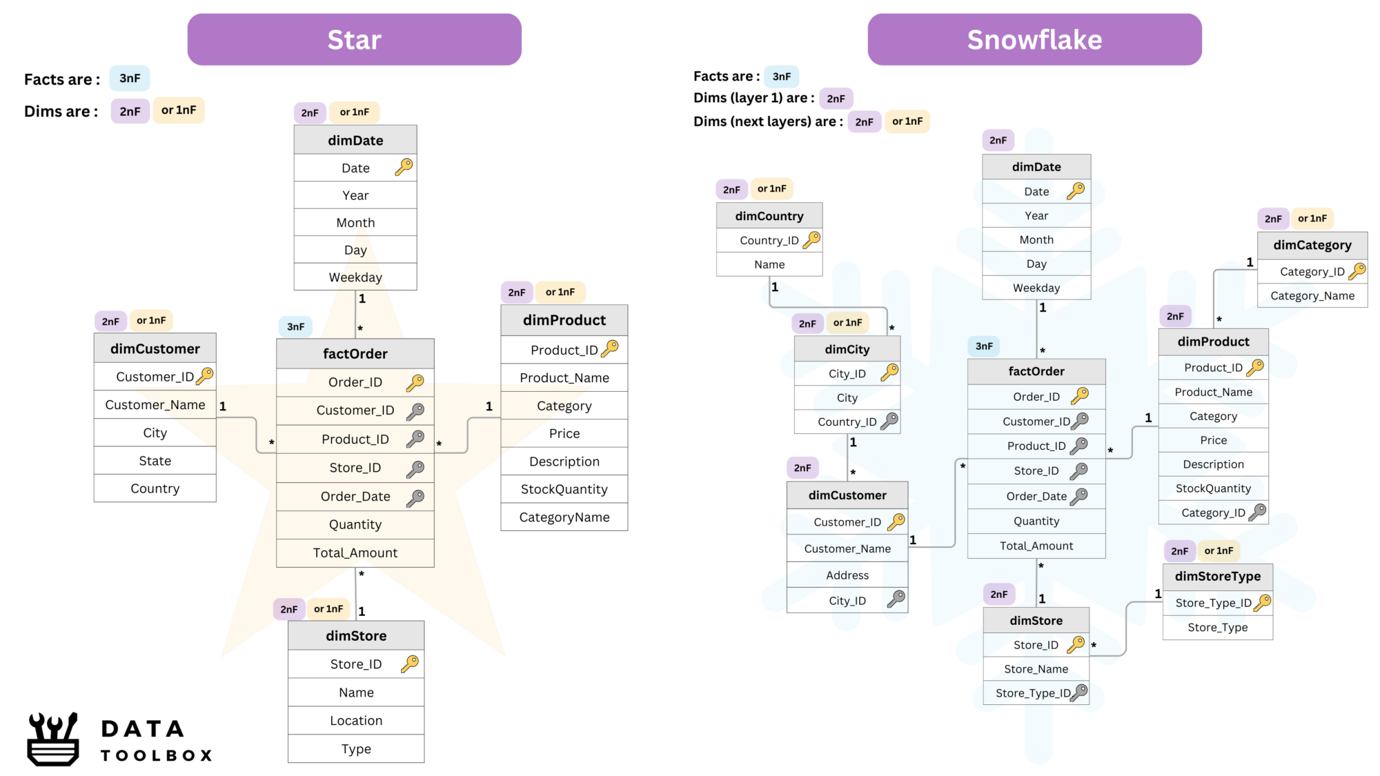
Building on these concepts, Kimball introduced three data modeling approaches that can be applied:
Star Schema
- A single fact table is surrounded by multiple dimension tables.
- Simplifies queries as joins are straightforward.
- Optimized for high-speed aggregation.
Snowflake Schema
- Extends the star schema by normalizing dimension tables.
- Reduces data redundancy but introduces more joins.
- Suitable for more complex analytical use cases.
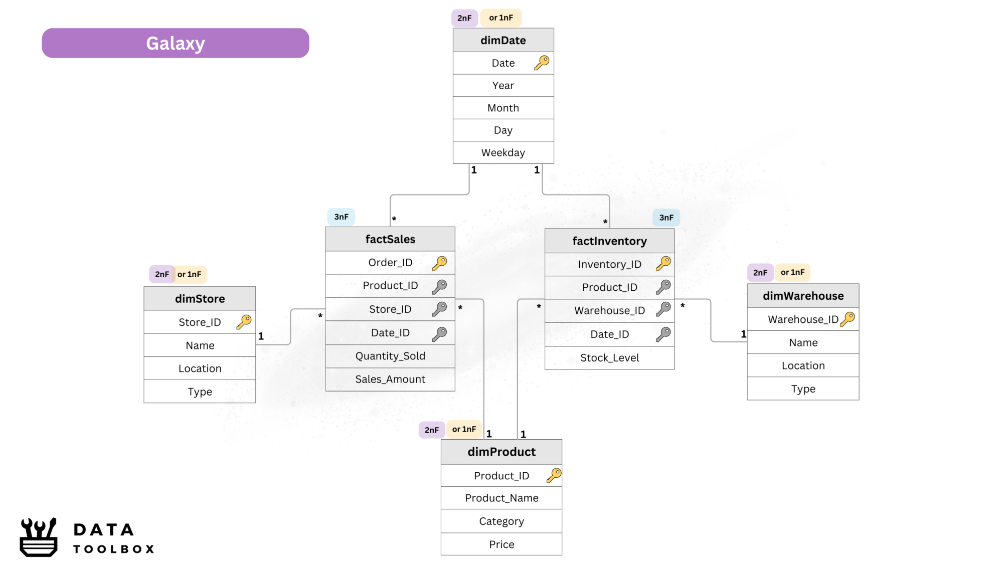
Galaxy Schema
- Also known as fact constellation.
- Supports multiple fact tables sharing common dimensions.
- Used for complex multi-fact analysis in large enterprises.
Today, dimensional modeling remains the standard approach for around 90% of companies (or maybe less—just a guesstimate 🤔) when designing their Gold layer, Data Marts and Semantic Layers.
Always transform and calculate data before it reaches the analytical layer to ensure dashboards and analytics run smoothly.
Golden rule of BI ✨
One of the key advantages of dimensional modeling is performance: by reducing the number of joins and enabling internal joins within dimension and fact tables, queries can run much faster. However, to preserve these benefits, certain pitfalls must be carefully avoided.
- Many-to-many cardinalities: These often lead to convoluted queries and slow performance.
- Direct fact-to-fact relationships: Fact tables should connect through shared dimensions instead of linking directly.
Data Vault Modeling
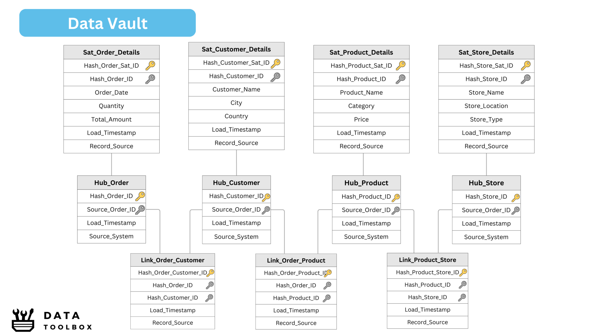
Data Vault is a hybrid approach that balances normalization and denormalization. It is designed for historical tracking, auditability, and scalability.
Key Components:
- Hubs: Represent core business entities (e.g., Customer, Product).
- Links: Capture relationships between entities.
- Satellites: Store descriptive attributes and historical changes.
Data Vault capitalizes on an insert-only pattern, utilizing hashing and load dates for tracking.
This architecture is well-suited for:
- Historical traceability: Every data point can be tracked over time, supporting compliance and governance needs.
- Highly scalable for large and evolving datasets and well-suited for integrating data from multiple sources.
- Event-driven architectures: As event streaming becomes more prevalent (and batch processing declines), the Data Vault model’s flexibility makes it an attractive choice for real-time or near-real-time data ingestion.
But my data model is different !
And this is fine 🤗 ! Theory offers a clear plan, but real projects often add tables and links that go beyond the plan, so when 10 fact tables connect many to many and dimensions keep growing, the model slows down and becomes hard to read.
A fix starts with purpose, so group fact tables that track the same grain, cut dimensions that do not help, and avoid one huge dashboard (the god object 🔱) that tries to show every metric at once. Give each report = 1 single business question, then test that question for speed and clarity.
How Are These Used in Real Life?
In the past, the go-to data modeling approach was heavily normalized, following the methodology introduced by Bill Inmon, often called the father of Data Warehousing. This approach aimed to create a normalized model from the source to the analytics layer, primarily because storage was expensive at the time (argument not relevant today, read more here).
On the other hand, Ralph Kimball advocated for the opposite philosophy: no centralized data warehouse, just denormalized Data Marts optimized for analytical workloads.
Fast forward 20 years, and the industry has evolved by blending both approaches into a practical compromise. A common approach to organizing data in modern environments is the three-layer structure :
🥉 Bronze Layer
- Stores unprocessed and raw data from different BUs, countries, etc.
- Useful for machine learning & analytics teams who need full-fidelity data.
🥈 Silver Layer
- Business and references datasets (e.g. products, sales, resources) integrated across multiple sources.
- Data is cleaned, deduplicated, historized and normalized.
- Ensures consistency and prepares data for further transformations.
- We typically use raw 3nF or Data Vault to model this layer.
🥇 Gold Layer
- Aggregated, summarized and enriched data used for a specific use case / data product.
- Optimized for analytics & reporting, using either Dimensional Models or Wide-Table.
Conclusion
So, what do you think? Convinced yet? We’ve covered a lot in this article: the vast constellation of data models 🪐 in the analytics world and how raw, unusable data is transformed into a polished dashboard presented to the company’s executive team.
👉 Wait, but do I have mutable or immutable data ? It’s not just a storage choice, it shapes your entire system. Explore the implications in Masterclass Data Modeling: How Data Changes Drive Schema Design.
👉 If you want to see how data models are applied in real life, check out this article: Blueprints for BI Data Modeling: Star, Hybrid, RLS, and SCD in Action.